Skip to content
AIS-01

AIS-01Fictional engineering demonstratorProof of concept

Satellite Mission Digital Twin

A mission-level digital twin of AIS-01, a fictional 250 kg satellite in a 550 km, 51.6° low Earth orbit. A Python engine propagates its orbital, electrical, thermal, attitude and communications state under coupled physical models and streams telemetry to a mission-control client several times a second.

Inject a fault at any moment and the consequence propagates through the physics rather than through a script — until the spacecraft’s own autonomy sheds load and enters safe mode without being told to. Nothing on screen is an animation.

Built by Omar Alsadaany. Financially supported by Alsadaany Industries.

Orbit altitude
550 km
Inclination
51.6°
Period
95.650 min
Spacecraft mass
250 kg
Injectable faults
8
Tests · assertions
198 / 516
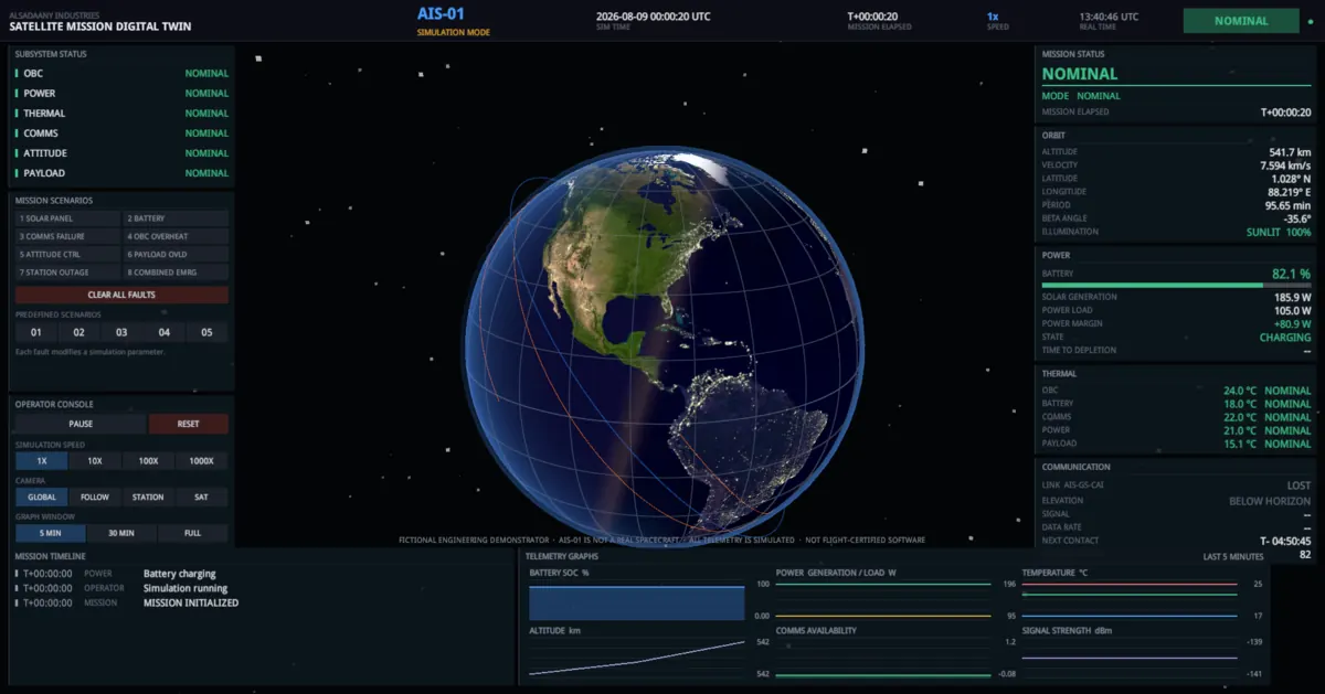
The AIS-01 mission-control console at T plus twenty seconds: Earth from orbit with the blue orbit path and orange ground track, six subsystems reading NOMINAL on the left, orbit, power, thermal and communications telemetry on the right, and the mission timeline and six live graphs across the bottom.

Mission-control console, nominal operations at T+00:00:20. Altitude 541.7 km, velocity 7.594 km/s, generation 185.9 W against a 105.0 W load, battery 82.1% and charging. Every value shown was integrated by the simulation, not authored.

Please read

AIS-01 is a fictional spacecraft. All telemetry is simulated. AIS-01 does not exist. Every parameter describing it was invented for this demonstration. This is not flight software, is not flight-certified, and does not represent any real satellite, mission, ground station or space agency. The physical constants are real published values; the spacecraft is not.

01Mission overview

A twin of a spacecraft that does not exist, built so everything about it behaves as though it does

A mission-level digital twin of a satellite that does not exist, built so that everything about it behaves as though it does.

AIS-01 is a fictional 250 kg satellite in a 550 km, 51.6° low Earth orbit. A Python simulation engine continuously propagates its orbital, electrical, thermal, attitude and communications state under physical models and streams the result over a WebSocket to a Unity mission-control client, which visualises the mission and sends operator commands back.

The distinction the project is built around is between a digital twin and a visualisation. The client computes no physics. It does not integrate, propagate, interpolate or invent a single displayed value — it renders telemetry and sends commands. If the engine stops, the client stops updating and says so, rather than coasting on an animation.

That constraint is what the whole demonstration rests on. There are no animation curves driving the satellite, no random values refreshed per frame, no hard-coded timeline and no placeholder graphs. Every number on screen originates in a state variable the simulation integrated.

What you can actually do with it

Open the browser build and you are looking at a mission-control console for a spacecraft already in flight. Mission time advances whether or not anyone is watching.

You can accelerate time from 1× to 1000× and the physics is identical either way. You can inject any of eight faults, each of which changes a real physical parameter rather than setting a status light, and then watch the consequence propagate through subsystems that are genuinely coupled to one another.

Push it hard enough and the spacecraft's own autonomy sheds the payload, inhibits the downlink and enters safe mode without being told to — and will not come out until the energy and thermal margins have actually recovered.

Why it was built

In a spacecraft, power, thermal, attitude and communications are one system. A pointing error changes solar generation, which changes battery state of charge, which changes what the vehicle can afford to run, which changes what it can downlink. Studying any of them alone produces an answer that is wrong in exactly the case that matters — the degraded one.

This project couples them, and then lets faults be injected into a running mission to see what the coupling actually does.

02Mission objectives

What the project set out to demonstrate

These are the properties the system was built to have, taken from the project’s own statement of intent. Each one names the constraint behind it, how it is implemented, and where in the repository that can be checked.

  1. 01Implemented

    Separate the simulation from every viewer of it

    Purpose
    A digital twin is only a twin if one component owns the state. Anything that recomputes state locally is a second, divergent model.
    Implementation
    The Python engine is authoritative. Telemetry crosses a single seam — `ITelemetryTransport` — and the entire client above that seam (views, camera, panels, graphs) does not know which platform or which engine it is running against.

    Evidencedocs/architecture.md

  2. 02Implemented

    Make faults propagate through physics, not through a script

    Purpose
    A fault that sets a status string proves nothing. A fault that changes a physical parameter and lets the consequences fall out is a test of whether the model is really coupled.
    Implementation
    Each of the eight faults changes exactly one physical parameter. None writes a status, schedules an outcome, or asserts a timeline. Battery degradation shrinks the pack rather than setting the state of charge — so the reported percentage rises at injection, then falls about 1.5× faster.

    Evidencesimulation-engine/app/simulation/faults.py

  3. 03Implemented

    Produce autonomous behaviour from state, not from a timeline

    Purpose
    Safe-mode entry is only meaningful if the spacecraft decides on it. Scheduling it removes the thing being demonstrated.
    Implementation
    Threshold rules with hysteresis on every one, evaluated against integrated state each tick. Safe mode is latched: entered at 20% state of charge, it will not clear until 45%, with thermals nominal and pointing inside limits, held for 120 s.

    Evidencesimulation-engine/app/simulation/autonomy.py

  4. 04Implemented, asserted in the test suite

    Make results independent of how fast you run the mission

    Purpose
    If accelerating time changed the outcome, time acceleration would be a way to reach a different mission rather than the same one sooner.
    Implementation
    Orbit propagation is analytical — state at time t is computed directly from the epoch elements, never accumulated. The integrated subsystems sub-step to a bounded 5 s maximum. A test asserts that a run at 1× and a run at 1000× agree.

    Evidencetests/test_engine.py::TestDeterminism::test_results_are_speed_independent

  5. 05Implemented

    Ship the limitations rather than conceal them

    Purpose
    A demonstrator that overstates its fidelity is worse than one that states it, because someone will eventually rely on it.
    Implementation
    A dedicated limitations document states what each model does not capture — no drag, no propulsion, a lumped thermal network rather than CFD or FE, a first-order attitude model, a link budget without rain fade or Doppler — and ships with the build.

    Evidencedocs/technical-limitations.md

  6. 06Implemented — desktop and WebGL builds produced

    Run the same interface anywhere, including a static host

    Purpose
    A demonstration nobody can open is not a demonstration. But a browser build cannot reach a Python process on a static host.
    Implementation
    Three interchangeable backends behind one transport interface: the Python engine over a threaded WebSocket on desktop, the Python engine over the browser WebSocket API via a .jslib bridge, and a C# port of the engine running in-process. The browser build defaults to the embedded engine, which is what makes it publishable.

    Evidenceunity-client/Assets/Scripts/Telemetry/

03Mission architecture

One component owns the state. Everything else is a viewer of it.

This is the property the whole demonstration rests on, and it is enforced structurally rather than by convention: the client has no code that could integrate, propagate or interpolate a value, and there is exactly one seam where telemetry crosses into it.

AIS-01 system architectureA Python simulation engine holds the authoritative state. The orbit propagator feeds solar and eclipse geometry, communications and attitude; those feed the power model, which exchanges heat with the thermal model. A fault manager mutates model parameters, an autonomy engine reads state and commands protective responses, and an event log records observed transitions. A runner advances the engine at 10 Hz and a connection hub broadcasts telemetry at 5 Hz through a FastAPI application exposing 17 REST endpoints and a WebSocket. Telemetry travels as JSON to a Unity mission-control client, which renders it and sends operator commands back over the same socket.SIMULATION ENGINEPython 3 · FastAPI · NumPy — the authoritative stateOrbitPropagatorJ2 · ECI / ECEF / geodeticSun & eclipseconical, with penumbraComms + stationvisibility · link budgetAttitudesaturating PD controlPowergeneration · batteryThermal6-node lumped networkcoupledFaultManagermutates model parametersAutonomyEnginereads state, commands responsesEventLogrecords observed transitionsSimulationRunneradvance(dt) at 10 Hz · TelemetryHistory ring buffer · ConnectionHub fan-out at 5 HzFastAPI · 17 REST endpoints · WS /ws/telemetry (state + commands)JSON telemetry · 5 Hzoperator commandsMISSION-CONTROL CLIENTUnity 6 — a viewer. Computes no physics.MissionLinkViewRigUI

Source · docs/architecture.md — component overview

Simulation engine

Python 3, FastAPI, NumPy — the authoritative state

  • OrbitPropagator — J2-perturbed Keplerian elements, ECI/ECEF/geodetic frames
  • solar_state — analytical ephemeris and conical eclipse geometry
  • PowerModel — generation, itemised loads, battery integration
  • ThermalModel — six-node lumped-capacitance network
  • CommsModel + GroundStation — visibility and link budget
  • AttitudeModel — saturating PD controller on three axes
  • FaultManager — mutates model parameters
  • AutonomyEngine — reads state, commands protective responses
  • EventLog — records observed transitions only

Runner & transport

A dedicated asyncio loop; request handlers never advance physics

  • SimulationRunner — advances the engine at 10 Hz
  • TelemetryHistory — ring buffer backing the graphs
  • ConnectionHub — WebSocket fan-out at 5 Hz, fire-and-forget
  • FastAPI — 17 REST endpoints plus /ws/telemetry

Mission-control client

Unity 6, built-in render pipeline — a viewer, not a model

  • MissionLink — owns the socket, parses frames on the main thread
  • View — Earth, satellite, orbit path, ground track, station, starfield
  • Rig — four camera modes
  • UI — mission-control console, panels, six live graphs

Why faults propagate

The subsystem models are not independent, and the couplings between them are what make an injected fault travel rather than sit in one panel. Each of these is a real term in a real equation, not a rule that watches for a condition.

Source · docs/architecture.md — coupling between subsystems

  • ThermalPower

    Hot photovoltaic cells lose output

  • AttitudePower

    Generation scales with the cosine of pointing error

  • ThermalAttitude

    A throttled on-board computer degrades control performance

  • PowerThermal

    Every watt consumed is dissipated as heat in the node that consumed it

  • CommsPower

    Transmitting costs 3.5× idle

  • OrbitEverything

    Eclipse gates generation and heat flux; geometry gates visibility

Three backends, one interface

The desktop and browser builds are the same client. Everything above the transport layer is identical and does not know which platform or which engine it is running on.

The browser cannot use the desktop transport — there are no .NET sockets and no threads in the sandbox — and on a static host it cannot reach the Python engine at all. That is why the embedded one exists.

EmbeddedBackend

Used when
Default, both builds
Engine
The C# port of the simulation, running in-process

NativeWebSocketTransport

Used when
Desktop with --engineHost
Engine
The Python engine, over a threaded WebSocket

WebGLWebSocketTransport

Used when
Browser with ?engineHost=
Engine
The Python engine, via the browser WebSocket API through a .jslib plugin

The wire format, and what constrained it

  • Telemetry is JSON over WebSocket at 5 Hz, shaped so Unity's built-in JsonUtility can consume it with no third-party dependency.
  • No dictionaries — collections are arrays of objects carrying a name field, because JsonUtility cannot deserialise a map and arrays keep row ordering stable.
  • No nullable value types — JsonUtility reads JSON null into a float as 0, which is indistinguishable from a real zero. Optional numbers carry an explicit −1 sentinel.
  • All unit conversion happens exactly once, at the serialisation boundary. The simulation package is strictly SI throughout; a conversion inside it would be a bug.

Source · docs/architecture.md · simulation-engine/app/models/schemas.py

04Spacecraft

AIS-01 — Alsadaany Industries Satellite Demonstrator 01

A 250 kg-class low Earth orbit smallsat. The vehicle is defined once, in a single configuration module, and every model reads its parameters from there — so there is no second, divergent copy of the spacecraft anywhere in the engine.

Every parameter below is fictional by the project’s own declaration, chosen to be internally consistent and typical of its class. The physical constants they are used with — WGS-84, IAU, IERS — are real published values.

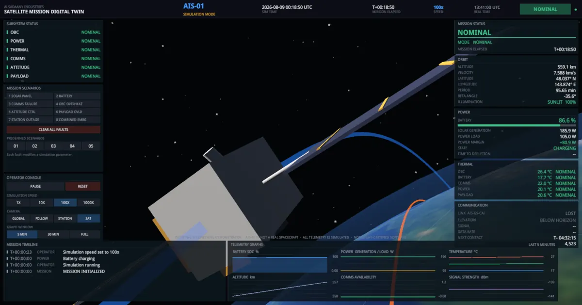
Close-up of the satellite body and solar array against black space, with Earth's limb at lower right.

AIS-01, close inspection

The close-inspection camera. The spacecraft model, the ground station, the orbit and ground-track lines, the starfield and the Earth shader are all generated procedurally from code — the only third-party assets in the project are NASA public-domain Blue Marble and Earth's City Lights imagery.

Mission elapsed
T+00:18:50
Altitude
559.1 km
Velocity
7.588 km/s
Battery
86.6 %

Vehicle identity

Designation
AIS-01
Mass
250kg
Class
LEO smallsat
Mission epoch
2026-08-09 00:00:00 UTC

Ground segment

Station
AIS-GS-CAI
Latitude
30.0444° N
Longitude
31.2357° E
Site altitude
75 m
Horizon maskBelow this the link is not attempted

AIS Ground Station Cairo is not a real facility. It is placed near Cairo because the location is recognisable; no real station’s coordinates, antenna or performance figures were used.

Bus & configuration

The vehicle is defined once, in a single configuration module, and every model reads its parameters from there. There is no second copy of the spacecraft anywhere in the engine.

Spacecraft mass
250kg
Structure thermal massThe bus dominates total heat capacity
46 000J/K
Radiator areaEffective area radiating to deep space
1.35
Radiator emissivitySecond-surface mirror / white paint
0.85
Solar absorptivityLow α/ε ratio, thermally controlled bus
0.32
Solar absorber areaProjected area receiving solar flux
1.05
Earth-facing areaProjected area seeing albedo and Earth IR
0.85

Source · simulation-engine/app/config.py

Electrical power

Sized so a nominal orbit closes its energy balance with a slightly positive orbit-average margin: the array must recover the eclipse depth-of-discharge during the sunlit arc, or the battery walks down over successive orbits.

Solar array areaTotal illuminated cell area, both wings
0.62
Cell efficiencyTriple-junction GaAs, beginning of life
0.295
Packing factorCell area / substrate area
0.92
Array tracking efficiencyTwo-axis gimbal: range limits, shadowing, deadband
0.88
Cell temperature coefficientAbove a 28 °C reference — this is the thermal → power coupling
−0.0021/K
Battery capacityNameplate Li-ion, beginning of life
520W·h
Initial state of charge
82%
Charge efficiencyCoulombic + conversion
0.95
Discharge efficiency
0.97
Max charge rateCharge-regulator limit
180W

Source · simulation-engine/app/config.py — PowerConfig

Electrical loads

Every watt on this list is also a thermal source. The load breakdown maps directly onto the thermal network's heat inputs, node for node.

On-board computer×0.60 in safe mode; throttled on thermal alarm
18W
Attitude controlReaction wheels and star tracker; ×0.75 in safe mode
22W
Comms — receiveReceiver always on
12W
Comms — transmitIncluding power-amplifier inefficiency
42W
PayloadImaging payload at nominal duty
45W
Bus overheadHarness losses and the power-distribution unit
8W
Battery heatersThermostatic, engaging below 8 °C
0 – 28W

Source · simulation-engine/app/config.py — PowerConfig

Thermal control

A six-node lumped-capacitance network: five component nodes coupled conductively to one structure node, which alone has a radiative view to space.

Battery heater setpointHeaters engage below this to protect the cells
8°C
Battery heater powerA real, switched electrical load
28W
Derating floorNode performance at its critical limit, from 1.0 at warning
0.35

Source · simulation-engine/app/config.py — ThermalConfig

Communications — S-band

A standard EIRP / free-space path loss / G-T / Eb-N0 chain, so received Eb/N0 responds correctly to slant range as the spacecraft rises and sets. Data rate is then selected adaptively from the achieved margin.

Downlink centre frequency
2.245GHz
Transmit power
5.0W
Spacecraft antenna gainNadir-facing patch
6.5dBi
Ground antenna gain1.2 m dish at S-band, η = 0.55
26.0dBi
System noise temperatureGround LNA plus sky noise, uncooled front end
320K
Implementation lossModem, pointing, polarisation mismatch
3.5dB
Atmospheric loss (zenith)Scaled by 1/sin(elevation)
0.6dB
Required Eb/N0Threshold for the coded waveform
4.5dB
Data rate rangeBelow the floor the link is declared unusable
64 kbps – 2.0 Mbps
On-board telemetry bufferStore-and-forward depth
20 000frames

Source · simulation-engine/app/config.py — CommsConfig

Attitude determination & control

A first-order rate/error model with a saturating PD controller on three decoupled axes — not a rigid-body dynamics simulation. The project documents this simplification explicitly.

Principal moments of inertiaIxx, Iyy, Izz
82 · 95 · 71kg·m²
Reaction-wheel torque authorityPer axis
0.028N·m
Proportional gain
0.055
Derivative gain
2.10
Disturbance torqueGravity-gradient plus aerodynamic, deterministic
3.2 × 10⁻⁵N·m
Pointing warning limitPayload imaging suspended
3.0°
Pointing critical limitTriggers autonomous safe mode
12.0°
Settled thresholdBelow this the controller reports LOCKED
0.5°

Source · simulation-engine/app/config.py — AttitudeConfig

Thermal network

Five component nodes exchange heat conductively with one structure node, which alone radiates to space. Above its warning limit a node’s performance derates linearly to 0.35 at its critical limit, so degraded performance is a measurable effect rather than a label.

Thermal node capacitances, conductances to the structure node, initial temperatures and warning and critical limits
NodeC · J/Kk · W/KInitial · °CWarning · °CCritical · °C
OBC2 6001.15245575
Battery18 5002.30184055
Comms3 1001.60225070
Power5 4002.05215572
Payload7 2002.60154560
Structure46 00012

Source · simulation-engine/app/config.py — ThermalConfig.nodes

05Orbital & mission parameters

A 550 km, 51.6° orbit, propagated analytically under secular J2

State at time t is computed directly from the epoch elements, never by accumulating steps. Propagation is therefore exact with respect to step size — which is what makes changing the simulation speed unable to change the trajectory.

There is no propulsion model and no atmospheric drag, so the orbit neither manoeuvres nor decays. Both omissions are documented in the project.

Orbital elements at epoch

AltitudeNominal, above the WGS-84 ellipsoid
550km
InclinationMid-inclination LEO
51.6°
EccentricityNear-circular, typical of an injected LEO smallsat
0.0012
RAAN at epoch
45.0°
Argument of perigee
0.0°
Mean anomaly at epoch
0.0°

Source · simulation-engine/app/config.py — OrbitConfig

Derived by the propagator

Orbital periodComputed by the propagator; checked against the analytic two-body period
95.650min
Ground-track driftWestward walk per revolution, a direct consequence of Earth rotation
−24.1° / rev
Nodal regressionSecular J2 effect at 51.6° inclination
≈ −4.6° / day
Earth angular radiusAs seen from 550 km — sets eclipse entry geometry
66.87°

Source · docs/simulation-model.md §1

Observed in the recorded run

Orbital velocityRange across the recorded run
7.576 – 7.594km/s
AltitudeRange across the recorded run
541.7 – 564.3km
Beta angleSun vector against the orbit plane, at the run epoch
−35.6°

Source · Marketing/screenshots — telemetry panel

Ground-track geometry at 51.6° inclinationA latitude–longitude grid with three successive orbit revolutions drawn as sine-like curves reaching 51.6 degrees north and south. Each revolution is displaced about 24 degrees west of the previous one because Earth rotates beneath the orbit during the 95.65 minute period. AIS Ground Station Cairo is marked at 30.04 degrees north, 31.24 degrees east, with a circle showing the region within which the spacecraft is in contact.60°S30°S30°N60°Nmax latitude = inclination 51.6°AIS-GS-CAI30.04°N 31.24°E · 5° maskSuccessive revolutions — each ~24.1° west of the lastStation coverage — contact occurs while the track is inside

Three successive revolutions at 51.6° inclination. Maximum latitude is bounded by the inclination — a geometric invariant no correct propagator can violate, and one the test suite asserts. Each pass is displaced about 24.1° west of the one before, because Earth rotates beneath the orbit during its 95.650-minute period.

That westward walk is why ground-station contacts arrive in clusters of consecutive orbits and then disappear for hours: the track marches away from Cairo and eventually comes back. A timer cannot reproduce that pattern, and the engine does not use one — visibility is computed from topocentric geometry against the 5° mask on every tick.

Time, and why speed does not change the result

The loop runs at 10 Hz of wall-clock time. At 1000× a single tick spans 100 s of mission time — far too long a step for the explicit integrators in the thermal and attitude models, so each request is split into sub-steps no longer than 5 s. Orbit propagation is immune to step size regardless.

The consequence is the one that matters for a demonstration: accelerating time to reach an interesting event does not change what happens when you get there.

Engine tick rateWall-clock period of the simulation loop
10Hz
Telemetry broadcastWebSocket fan-out to every connected client
5Hz
Max integration sub-stepBounds the explicit integrators at high time acceleration
5s
Time acceleration
1× · 10× · 100× · 1000×
History ring bufferBacks the graphing endpoints
24 000samples
Random seedFixed — identical seed produces an identical run
20260809

Source · simulation-engine/app/config.py — SimulationConfig

06Simulation

What is actually being simulated, and what happens when you break it

The engine computes orbit, illumination, power, thermal, communications and attitude state every tick, in an order that encodes physical causality. What follows are frames from a recorded run, each paired with the mechanism that produced it and the telemetry it carries.

Fault injection

Each of the eight faults changes a physical parameter. None writes a status string, and none schedules an outcome. Injecting one changes a number and the simulation carries on; what follows is whatever the physics and the autonomy rules produce.

Battery degradation is the clearest illustration. It does not set the state of charge — it shrinks the pack. Stored energy is unchanged, so the reported percentage rises at injection, then falls about 1.5× faster. Nothing about that was scripted.

Source · simulation-engine/app/simulation/faults.py

  • 1

    Solar Panel Degradation

    Array factor 1.00 → 0.45

  • 2

    Battery Degradation

    Usable capacity → 65% of nameplate

  • 3

    Communication Failure

    Radio marked failed → LINK FAILURE

  • 4

    OBC Overheating

    +65 W into the OBC thermal node

  • 5

    Attitude Control Failure

    Wheel torque → 0, plus a 0.66 N·m·s momentum dump

  • 6

    Payload Overload

    Payload draw ×2.6 — 45 W → 117 W

  • 7

    Ground Station Outage

    Station out of service; passes occur but cannot be worked

  • 8

    Combined Emergency

    Faults 1 + 2 + 3 + 4 together

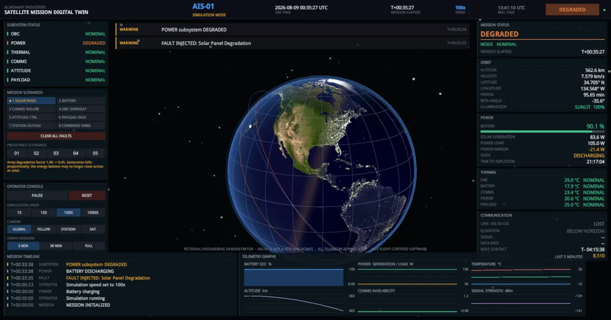
Console with the SOLAR PANEL fault button highlighted, mission status DEGRADED in amber, solar generation 83.6 watts against a 105 watt load and a negative power margin.

Fault 1 — solar panel degradation

The array degradation factor is set from 1.00 to 0.45. Generation falls from 185.9 W to 83.6 W against an unchanged 105.0 W load, so the margin inverts to −21.4 W and the battery starts discharging. Nothing set a status: POWER went DEGRADED because the energy balance stopped closing.

Mission elapsed
T+00:35:27
Generation
83.6 W
Load
105.0 W
Margin
−21.4 W
State
DISCHARGING
Time to depletion
21:17:04
Status
DEGRADED

Autonomous response

Threshold rules with hysteresis on every one, because a spacecraft sitting on a trip point would otherwise oscillate every tick. The response is graduated: load is shed before the mode changes, because shedding may resolve the condition without the operational cost of a safe-mode entry.

Safe mode is latched. If a fault leaves the energy balance unable to reach 45%, the spacecraft stays in safe mode indefinitely and waits for the ground — which is what makes clearing the fault meaningful.

Source · simulation-engine/app/simulation/autonomy.py

  • State of charge ≤ 30%

    Shed payload
  • State of charge ≤ 20%

    Shed payload, inhibit downlink, SAFE MODE
  • OBC at warning limit

    Throttle processing to 80%
  • OBC at critical limit

    Throttle to 55%, shed payload, SAFE MODE
  • Battery outside survival limits

    Shed payload, SAFE MODE
  • Pointing error ≥ 3°

    Suspend payload imaging
  • Pointing error ≥ 12°

    SAFE MODE
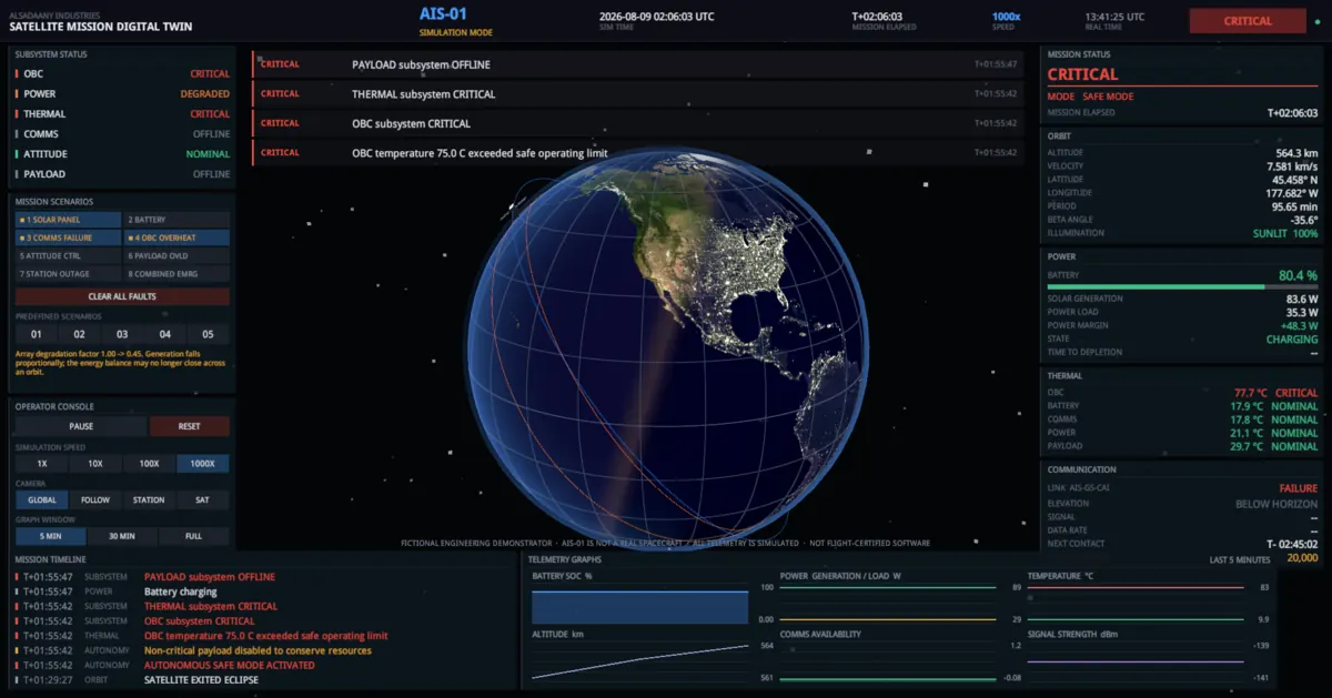
Console in safe mode: mission status CRITICAL, mode SAFE MODE, OBC at 77.7 degrees Celsius in red, payload and comms subsystems offline, and a timeline entry reading AUTONOMOUS SAFE MODE ACTIVATED.

Autonomous safe-mode entry

The OBC crossed 75 °C and the spacecraft entered safe mode by itself. The timeline records the sequence in order: OBC temperature exceeded safe operating limit, non-critical payload disabled to conserve resources, AUTONOMOUS SAFE MODE ACTIVATED. Payload and comms read OFFLINE. Load has dropped from 105.0 W to 35.3 W and the margin is positive again at +48.3 W — the vehicle shed its way back to a closing energy balance without being commanded to.

Mission elapsed
T+02:06:03
Mode
SAFE MODE
OBC
77.7 °C
Load
35.3 W
Margin
+48.3 W
Payload
OFFLINE
Queued frames
20 000 (saturated)

Predefined scenarios are starting conditions, not scripts

Applying a scenario resets the mission, optionally positions the spacecraft at an interesting point in its orbit, optionally sets the battery to a chosen state of charge, and injects a set of faults. From that instant the simulation simply runs. Nothing schedules an outcome or asserts a timeline.

The expected behaviour recorded against each scenario is a prediction, shown in the interface so a viewer can check the engine against it — not an instruction to the engine. Change the array area in the configuration and Power Crisis may no longer reach safe mode at all.

01

Nominal Mission

Healthy spacecraft in its design orbit. No faults injected.

Expected behaviour

Battery cycles between roughly 80% and 100% across each orbit. Generation drops to zero through eclipse and recovers on sunrise. Ground-station contacts occur in clusters of consecutive orbits separated by multi-hour gaps as the ground track walks away from Cairo.
02

Power Crisis

Spacecraft enters eclipse with a degraded solar array and a partly depleted battery.

Expected behaviour

On sunrise the degraded array cannot fully recover the depth of discharge, so successive orbits walk the state of charge down. As it crosses 30% the payload is shed; at 20% the spacecraft enters safe mode. Recovery follows only once the reduced load lets the array rebuild charge past 45%.

03

Communication Failure

Transceiver hardware fails while the spacecraft is otherwise healthy.

Expected behaviour

The link reports LINK FAILURE rather than LINK LOST, so the cause is distinguishable from a routine horizon crossing. Telemetry queues on board and the backlog grows across every missed pass. Clearing the fault restores the link at the next geometric contact, and the backlog then drains at the achieved data rate.

04

Thermal Anomaly

Parasitic heat load in the on-board computer.

Expected behaviour

OBC temperature rises on the node's own ≈38-minute time constant through its 55 °C warning limit toward the 75 °C critical limit. Processing is throttled progressively as it climbs, which degrades attitude-control performance as a second-order effect. Crossing the critical limit triggers safe mode.

05

Emergency Mission

Combined failure: degraded array, degraded battery, communications failure and OBC overheating.

Expected behaviour

Multiple independent failure paths converge. Power depletes faster than in the Power Crisis scenario because reduced capacity compounds reduced generation; the OBC heats toward its critical limit in parallel; and no telemetry can be downlinked while it happens.

Source · simulation-engine/app/scenarios/definitions.py

Telemetry and recorded history

Six graphs plot the engine’s own ring buffer: battery state of charge, generation against load, temperatures, altitude, link availability and signal strength. Eclipse periods are shaded behind them. An empty buffer draws an empty graph and says so.

The mission timeline beside them is generated the same way — every entry is an edge-detected state transition, logged once at the moment it happened. No timestamp is hard-coded.

Telemetry frame contents

  • Orbit — position, velocity, altitude, latitude/longitude, ground track, period, phase, beta angle
  • Illumination — sun vector and conical eclipse fraction
  • Power — generation, state of charge, itemised loads, margin, time to depletion
  • Thermal — five component node temperatures against warning and critical limits
  • Communications — visibility, link budget, signal strength, adaptive data rate, contact windows, backlog
  • Attitude — roll/pitch/yaw error, body rates, control state
  • Health — six subsystem states, mission mode, mission status
  • Autonomy — load shedding, downlink inhibit, safe-mode entry and recovery
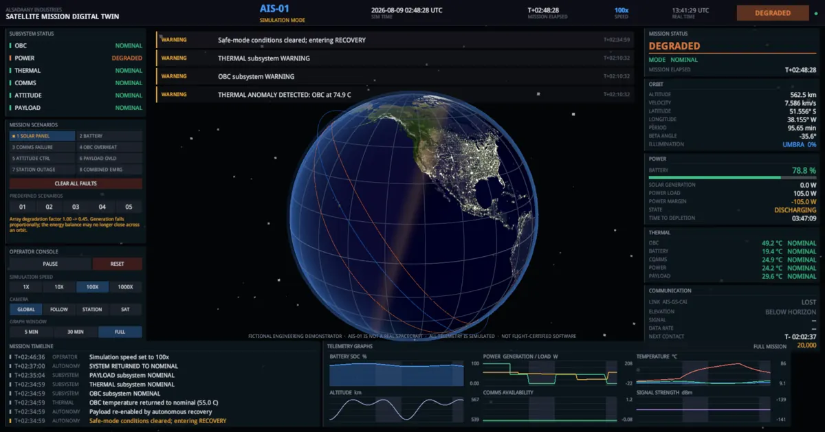
Console with the full-mission graph window selected, showing six telemetry plots over the whole run with shaded vertical bands marking eclipse periods.

Full-mission history

The graph window switched to FULL MISSION. This is recorded history from the engine's ring buffer, not a redrawn summary: battery state of charge, generation against load, temperatures, altitude, link availability and signal strength. The shaded vertical bands are eclipse periods. The altitude trace shows the orbital oscillation over the run; the temperature trace shows the OBC excursion and its recovery.

Mission elapsed
T+02:48:28
Graph window
FULL MISSION
Altitude range
539 – 567 km
Battery
78.8 %
OBC
49.2 °C

07Technical systems

The subsystems, and what each one actually models

Nine implemented systems. Each entry states the model, the reasoning behind it, and the file it lives in — so any claim here can be checked against the code rather than taken on trust.

There is no propulsion section because there is no propulsion model. The project states this plainly, and nothing is listed here that does not exist.

01

Orbital mechanics

Mean Keplerian elements advanced under secular J2 perturbation, with the osculating state evaluated analytically at any epoch.

Source · simulation-engine/app/simulation/orbit.py

Kepler's equation is solved by Newton–Raphson — three to four iterations at LEO eccentricities — and the perifocal state rotated to ECI by the classical 3-1-3 sequence.

J2 is roughly a thousand times larger than every other perturbation in LEO and produces the two effects an operator actually sees: the ground track walking west each revolution, and the orbit plane regressing.

State at time t is computed directly from the epoch elements, never by accumulating steps. Propagation is therefore exact with respect to step size, which is what makes changing the simulation speed unable to change the trajectory.

Frames: ECI (TEME-like — precession and nutation are not modelled), ECEF via a single GMST rotation using the IAU-1982 polynomial, and geodetic on the WGS-84 ellipsoid via Bowring's method plus one Newton refinement.

Perturbation model
Secular J2
Propagation
Analytical, not integrated
Geodetic round-trip error
~1 × 10⁻¹³ °
Speed vs vis-viva
Agrees to 1 × 10⁻⁹ relative

02

Solar geometry & eclipse

A conical shadow with a true penumbra, computed from the apparent angular radii of the Sun and Earth — not a binary in-shadow flag.

Source · simulation-engine/app/simulation/sun.py

The spacecraft's illumination is the fraction of the solar disc not occulted by the Earth, derived from two-circle lens-area geometry across four regimes: full sun, umbra, annular and penumbra.

This matters because a 550 km orbit crosses the penumbra in ten to fifteen seconds. A cylindrical shadow would snap generation from 100% to 0% in a single tick, producing a square-wave power profile no operator would find credible.

The solar ephemeris is the Astronomical Almanac low-precision series — accurate to about 0.01° in direction, roughly three orders of magnitude better than the array-pointing model it feeds, so it is not the limiting error.

Beta angle — the angle between the Sun vector and the orbit plane — is displayed because it explains why eclipse duration changes over days of simulated time.

Shadow model
Conical, with penumbra
Measured penumbral width
0.517°
Sun's angular diameter
0.532°
Ephemeris accuracy
~0.01° in direction

03

Electrical power

Generation as an area–efficiency–incidence product with a photovoltaic temperature coefficient, integrated into a battery with separate charge and discharge efficiencies.

Source · simulation-engine/app/simulation/power.py

Generation is P = A · η · f_pack · G · Φ · cos θ · D · k_T, where Φ is the illumination fraction from the eclipse model and k_T carries the cell temperature coefficient — this is the thermal-to-power coupling made explicit.

Array temperature is solved at radiative equilibrium rather than integrated: a deployed panel has very small thermal mass relative to its radiating area and settles in seconds.

The battery is an explicit Euler integrator on stored energy. Capacity is 520 W·h nameplate multiplied by health, and state of charge is energy divided by capacity.

Degradation therefore preserves energy, not state of charge. Shrinking usable capacity leaves the stored joules untouched, so the reported percentage rises at the instant of injection and then falls about 1.5× faster under the same load.

Array area
0.62 m²
Cell efficiency
0.295 (3J GaAs)
Battery capacity
520 W·h
Nominal load
105 W observed

04

Thermal control

Six lumped capacitances — five component nodes coupled conductively to one structure node, which alone radiates to space.

Source · simulation-engine/app/simulation/thermal.py

Each component node integrates C·dT/dt = Q + k(T_structure − T_node), where Q is the electrical power dissipated in that component. Essentially all electrical power a spacecraft consumes ends up as heat, so the load breakdown maps directly onto the thermal sources.

The structure node adds three environmental fluxes — direct solar and Earth albedo, both gated by illumination, and Earth infrared, present day and night — and radiates against the 2.725 K cosmic background.

Earth IR is why the spacecraft settles at a survivable temperature during eclipse rather than cooling toward 2.7 K.

Above its warning limit a node's performance derates linearly to 0.35 at its critical limit, which makes 'degraded performance' a measurable effect rather than a label. A throttled on-board computer degrades attitude-control performance as a second-order consequence.

Nodes
6 (5 components + structure)
OBC time constant
≈ 38 min
OBC limits
55 °C warning / 75 °C critical
Structure capacity
46 000 J/K

05

Communications

Topocentric visibility against a horizon mask, plus a full EIRP / path-loss / G-T / Eb-N0 link budget with elevation-scaled atmospheric loss.

Source · simulation-engine/app/simulation/comms.py

Visibility is computed from geometry, never a timer. The station-to-spacecraft vector is rotated into the station's local East-North-Up frame and the elevation read off; the link is attempted only above the 5° horizon mask.

That is why contacts occur in clusters of consecutive orbits separated by multi-hour gaps as the ground track walks away from Cairo — a pattern a timer cannot reproduce. Pass boundaries are found by coarse scan plus bisection, landing on the mask to within 0.05°.

Atmospheric loss scales as 1/sin(elevation) — the flat-slab approximation — so a 6° pass is meaningfully worse than one overhead. The achievable rate is clamped to the modem's 2 Mbps ceiling, which is why the rate holds at maximum through the middle of a good pass and rolls off near acquisition and loss of signal.

Telemetry accumulates on board at four frames per second whenever the link is down and drains at the achieved rate when it is up, so a long outage leaves a backlog that takes real contact time to clear.

Band
S-band, 2.245 GHz
Horizon mask
Pass-boundary precision
0.05°
Buffer depth
20 000 frames

06

Guidance, navigation & control

Three decoupled single-axis pointing-error dynamics with a saturating PD controller and deterministic disturbance torques.

Source · simulation-engine/app/simulation/attitude.py

Integration is semi-implicit (symplectic) Euler — rate first, then angle from the updated rate. Explicit Euler would inject energy and slowly diverge even with a healthy controller.

The disturbance torque is deterministic, modelled as fixed-phase harmonics of the argument of latitude — gravity-gradient at twice per revolution, aerodynamic at once per revolution. It is a repeatable function of where the spacecraft is, not a random draw, so two runs from the same configuration produce identical attitude histories.

A healthy wheel has roughly 875× margin over the disturbance environment — 0.028 N·m against 3.2 × 10⁻⁵ N·m — so degrading it to even a few percent still holds attitude comfortably, and the test suite asserts exactly that.

The physically meaningful failure is therefore a wheel that stops producing torque and dumps its stored momentum into the body, after which nothing can arrest the resulting rate. That is what the attitude fault does.

Control law
Saturating PD, per axis
Integrator
Semi-implicit Euler
Wheel margin over disturbance
≈ 875×
Momentum dump on failure
0.66 N·m·s

07

Flight software — autonomy & FDIR

Threshold rules with hysteresis on every one, producing a graduated response: load is shed before the mode changes.

Source · simulation-engine/app/simulation/autonomy.py

Shedding may resolve the condition without the operational cost of a safe-mode entry, so the response ladder tries that first.

Safe mode is latched. It is entered at 20% state of charge but will not clear until 45%, thermals are nominal and pointing is inside the warning limit — held for 120 s. A payload shed for power reasons is not restored until state of charge recovers a further 8% above the threshold that shed it.

The consequence is deliberate: if a fault leaves the energy balance unable to reach 45%, the spacecraft stays in safe mode indefinitely and waits for the ground. That is correct behaviour, and it is what makes clearing a fault in the demonstration mean something.

The project is explicit that this is illustrative. Real spacecraft FDIR involves layered monitors, command authorisation, redundancy management and recovery sequencing that this does not attempt.

Safe-mode entry
20% SOC
Safe-mode release
45% SOC, held 120 s
Payload restore margin
+8% above shed threshold
Hysteresis
On every rule

08

Mission event log

A timeline generated from observed state transitions. No entry is ever scheduled or hard-coded.

Source · simulation-engine/app/simulation/events.py

An edge detector reports only transitions, so 'battery below 30%' is logged once, at the moment it happened, rather than on every subsequent tick while the condition holds.

Both directions of a condition must be queried through a single edge() call — calling rising() and then falling() on the same key silently breaks the falling edge, because each records the new value as a side effect.

That was a real bug in development. It suppressed every 'satellite exited eclipse' event until it was found by asserting that eclipse entries and exits balance.

Generation
Edge-detected transitions
Scheduled entries
None
Regression guard
Eclipse entries must balance exits

09

Ground segment & operator interface

A mission-control console built entirely in code at runtime: four camera modes, subsystem status, telemetry panels, a live event timeline and six graphs.

Source · unity-client/Assets/Scripts/

The saved Unity scene contains exactly one GameObject with a bootstrap component. Everything else is constructed in code, so the scene can be reviewed in a diff, regenerated from a clean checkout, and cannot break when a .unity file is re-serialised by a different editor version.

Earth's rotation is not recomputed client-side. It is recovered from the azimuth difference between the ECI and ECEF positions of the same frame, so the planet's orientation can never drift away from the server's and put the ground track in the wrong place.

One Unity unit is 1000 km. Earth's equatorial radius is 6.378 units; a 550 km orbit sits at 6.928. The spacecraft model is drawn at exaggerated scale so it is visible — its position is exact, its size is not.

The interface refreshes at 10 Hz against a 5 Hz telemetry stream, writing only to existing text and image components. Nothing is allocated or instantiated per frame.

Scene objects in the saved scene
1
Camera modes
4
Live graphs
6
Per-frame allocation
None

Not modelled

What these systems deliberately do not capture

Where a full-fidelity model was impractical for a proof of concept, the simplest scientifically coherent model was implemented and the limitation documented — rather than concealed behind an animation.

Source · docs/technical-limitations.md §3

  • Atmospheric drag and orbital decay

    A real 550 km orbit loses roughly 1–3 km/month at moderate solar activity. Not modelled, so the orbit does not decay.

  • Propulsion

    There is no propulsion model. The orbit cannot be changed from the interface.

  • Higher-order geopotential, third-body gravity, solar radiation pressure

    J2 dominates LEO over the timescales simulated. Position is good to roughly a kilometre over hours and degrades over days.

  • CFD or finite-element thermal analysis

    No spatial discretisation, no view factors, no fluid. Temperatures are representative, not predictive.

  • Quaternion kinematics, wheel momentum accounting, sensor models

    Attitude is a first-order decoupled error model, not rigid-body dynamics.

  • Rain fade, Doppler, multipath, protocol overhead

    The link budget is a clean EIRP/FSPL/G-T/Eb-N0 chain with an elevation-scaled atmospheric term.

  • Cell-level electrochemistry and coulomb counting

    State of charge is energy-based. No voltage curves, internal resistance or ageing over cycles.

  • Authentication and transport security

    The API is unauthenticated with permissive CORS, built to run on loopback for a demonstration. Explicitly not for exposure to an untrusted network.

08Engineering data

Figures that can be checked

Each of these came from the repository or from running it. Where the project does not measure something, no number appears here — there is no spacecraft power budget in watts against a mission requirement, no pointing accuracy in arcseconds, no reliability figure, because none of those exist to be quoted.

198

Engine tests passing

Python suite, 6 modules, 33 test classes. Verified by running it: 198 passed, 0 failed.

516

Client assertions passing

The C# port of the engine, checked against the same independently-derived physics.

18 639

Lines of engineering code

6 280 Python engine · 10 258 C# client across 42 files · 2 101 lines of tests.

95.650min

Orbital period at 550 km

Computed by the propagator and checked against the analytic two-body period.

8

Injectable faults

Each changes one physical parameter. None writes a status or schedules an outcome.

15

Steps in the tick sequence

A fixed order, because the order encodes physical causality.

10 / 5Hz

Engine rate / telemetry rate

The simulation advances at 10 Hz; telemetry fans out to every client at 5 Hz.

1000×

Maximum time acceleration

Results are speed-independent — the test suite asserts a 1× run matches a 1000× run.

09Testing & validation

Checked against physics derived independently of the implementation

The interesting question for a simulation is not whether it runs, but whether it reproduces things it was never told. The checks below are the ones that answer that: each is a physical constraint derived outside the code, asserted against what the propagator and the models actually produce.

Verification checks

Critical inclination — apsidal drift → 0

63.435°

The inclination at which J2 stops rotating the line of apsides. Recovering it means the J2 secular terms carry the right coefficients, not merely the right shape.

Sun-synchronous inclination — 360°/year nodal drift

≈ 97.6°

A second, independent constraint on the same terms, from the opposite direction. Both are recovered from the propagator, not configured into it.

Speed against vis-viva

Agrees to 1 × 10⁻⁹ relative

v = √(μ(2/r − 1/a)) is an exact two-body identity. Agreement at this level says the perifocal-to-ECI rotation preserves the energy.

Orbital period at 550 km

95.650 min

The directly checkable consequence of the semi-major axis and μ.

Ground-track drift per revolution

−24.1°

Follows from Earth's rotation during one period. It is why contacts cluster and then disappear for hours.

Geodetic round-trip

~1 × 10⁻¹³ °

Cartesian → geodetic → Cartesian on the WGS-84 ellipsoid. Bounds the error in every latitude and longitude the console displays.

Penumbra angular width

0.517° vs the Sun's 0.532° disc

Matches to within 3%. A cylindrical shadow model has zero penumbral width by construction, so this is the check that distinguishes the two.

Solar declination at solstices

± 23.44°

Validates the ephemeris obliquity, which sets beta angle and therefore eclipse duration.

Free-space loss on doubling range

6.02 dB

The inverse-square law, exactly. Confirms the link budget responds correctly to slant range through a pass.

Maximum latitude

≤ inclination

A geometric invariant no correct propagator can violate.

Source · docs/simulation-model.md · tests/test_orbit.py · tests/test_sun_eclipse.py

Test suites

198

Python engine tests

Run against a clean checkout for this write-up: 198 passed, 0 failed.

516

C# client assertions

The embedded engine checked against the same independently-derived physics. 516 passed, 0 failed.

How they are run

python -m pytest
Tools/unity.sh selftest

Coverage by module

Python test modules, the number of tests each contains, and what they cover
ModuleTestsCovers
test_engine.py50Tick order, determinism, speed-independence, safe-mode entry and recovery, event generation
test_api.py42Every REST endpoint and the WebSocket contract, including reset confirmation
test_subsystems.py41Power generation and battery integration, the thermal network and its thresholds, attitude control and its failure
test_orbit.py29Propagation, frame transforms, geodetics, critical and sun-synchronous inclinations
test_comms.py24Visibility geometry, link budget, contact prediction, store-and-forward backlog
test_sun_eclipse.py12Solar ephemeris, conical shadow geometry, penumbra width, beta angle

How the demonstration was recorded

The capture harness drives the demonstration through the same commands the operator buttons use. It has no privileged path into the simulation. For the fault-response frames it waits on telemetry conditions rather than fixed timings — so a still labelled “safe mode” was taken because the spacecraft had actually entered safe mode.

If a condition is never reached, the manifest records [CONDITION NOT MET - TIMED OUT] rather than presenting the frame as if it had been.

Source · Marketing/README.md · unity-client/Assets/Scripts/App/MissionCapture.cs

10Results

One recorded run, from nominal to safe mode and back

Everything below came from a single continuous run of the demonstration flow. Each result states what was measured and under what conditions, and points at the frame it can be read off. No transition was produced by the capture script.

  1. R01

    Autonomy closed an energy balance it was not commanded to close

    Measured
    At T+01:13:02, in eclipse with a degraded array, the power margin was −89.4 W against a 105 W nominal load. At T+02:06:03, after autonomous safe-mode entry shed the payload and inhibited the downlink, load read 35.3 W and the margin read +48.3 W.
    Conditions
    Faults 1, 3 and 4 active simultaneously. No operator command was issued between those two frames other than time acceleration.

    EvidenceFrames 08 and 10 of the recorded run

  2. R02

    The safe-mode latch held for 27 minutes after the cause was removed

    Measured
    Faults were cleared at T+02:07:50. The latch did not release until T+02:34:59 — 27 min 09 s later — and the system returned to nominal at T+02:37:00, 29 min 10 s after the operator's action.
    Conditions
    Release requires 45% state of charge, nominal thermals and pointing inside the warning limit, held for 120 s. The OBC had to cool from 77.7 °C on its own ≈38-minute time constant before the thermal condition could be met.

    EvidenceFrames 11 and 12, and the on-screen mission timeline

  3. R03

    A fault changed a parameter; the status followed from the physics

    Measured
    Injecting solar panel degradation moved generation from 185.9 W to 83.6 W against an unchanged 105.0 W load. The margin inverted to −21.4 W, the battery state changed to DISCHARGING, and POWER reported DEGRADED.
    Conditions
    Sunlit arc, all other subsystems nominal. The fault sets the array degradation factor to 0.45 and nothing else.

    EvidenceFrames 01 and 06

  4. R04

    Loss of signal and loss of hardware stayed distinguishable throughout

    Measured
    Before the comms fault the link read LOST with elevation BELOW HORIZON and a counted-down next contact. After injection it read FAILURE. The on-board backlog grew 10 870 → 17 530 → 19 229 frames and saturated at the 20 000-frame buffer depth.
    Conditions
    The store-and-forward buffer accumulates at four frames per second while the link is down and drains at the achieved data rate when it is up.

    EvidenceFrames 05, 07, 08, 09 and 10

  5. R05

    The propagator reproduced physics it was never told

    Measured
    Critical inclination recovered at 63.435°, sun-synchronous inclination at ≈97.6°, speed agreeing with vis-viva to 1 × 10⁻⁹ relative, and a modelled penumbra 0.517° wide against the Sun's 0.532° disc.
    Conditions
    Checks derived independently of the implementation and asserted in the test suite, not configured into the propagator.

    Evidencetests/test_orbit.py, tests/test_sun_eclipse.py

The recorded run, frame by frame

Mission-elapsed time is the clock on that frame, and every reading in a row was taken from that same frame. Where an event happened earlier than the frame that documents it, the event’s own timeline timestamp is given — the two are not conflated.

Each captured frame of the demonstration run with its mission-elapsed time, the event it documents, flight-software mode, mission status, battery state of charge, on-board computer temperature and link state
Mission elapsedWhat the frame documentsModeStatusSOCOBCLink
T+00:00:20Mission nominal, 1×NOMINALNOMINAL82.1 %24.0 °CLOST
T+00:02:15Time acceleration to 100×NOMINALNOMINAL82.6 %24.2 °CLOST
T+00:10:22Follow cameraNOMINALNOMINAL84.6 %25.2 °CLOST
T+00:18:50Spacecraft inspectionNOMINALNOMINAL86.6 %26.4 °CLOST
T+00:27:19Ground-station viewpointNOMINALNOMINAL88.7 %27.7 °CLOST
T+00:35:27Solar panel degradation active — injected T+00:33:35NOMINALDEGRADED90.1 %29.0 °CLOST
T+00:45:17Communication failure active — injected T+00:43:45NOMINALCRITICAL89.5 %30.5 °CFAILURE
T+01:13:02OBC overheating in eclipse — injected T+00:53:36NOMINALCRITICAL84.2 %55.6 °CFAILURE
T+01:20:07Past the 55 °C warning limit — crossed T+01:12:14NOMINALCRITICAL82.1 %60.4 °CFAILURE
T+02:06:03Autonomous safe mode — activated T+01:55:42SAFE_MODECRITICAL80.4 %77.7 °CFAILURE
T+02:27:14Latch still held — faults cleared T+02:07:50SAFE_MODECRITICAL83.2 %59.8 °CLOST
T+02:44:50Recovered — released T+02:34:59, nominal T+02:37:00NOMINALDEGRADED80.1 %50.8 °CLOST
T+02:48:28Full-mission graph windowNOMINALDEGRADED78.8 %49.2 °CLOST

Source · Marketing/screenshots — capture-manifest.csv and the frames themselves

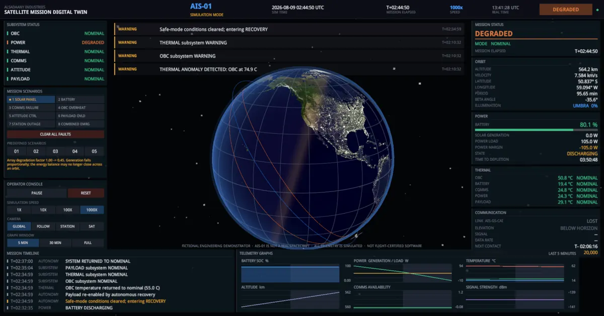
Console back in NOMINAL mode with all subsystems green except POWER, and a timeline showing safe-mode conditions cleared and the system returned to nominal.

Recovered to nominal

Safe-mode conditions cleared at T+02:34:59 — 27 minutes of mission time after the operator cleared the faults — and the system returned to nominal two minutes later at T+02:37:00. The timeline shows the release in sequence: OBC temperature returned to nominal, payload re-enabled by autonomous recovery, safe-mode conditions cleared, system returned to nominal. Status stays DEGRADED because the array fault is still active.

Mission elapsed
T+02:44:50
Mode
NOMINAL
Safe mode released
T+02:34:59
Returned to nominal
T+02:37:00
OBC
50.8 °C
Status
DEGRADED

12How it works

From engine start to earned recovery

The path a mission takes through the system, and the fixed order the engine works in every tick — because that order is what encodes physical causality.

  1. 01

    The engine starts

    Mission time begins advancing immediately, with or without a client attached. The vehicle is initialised from a single configuration module at a fixed epoch, so a fresh checkout produces the same mission every time.

  2. 02

    The client connects

    Desktop or browser, the same interface. It resolves an endpoint, opens a WebSocket and receives a full telemetry frame immediately — so there is no partial-state window. Starting the client late simply joins a mission already in progress.

  3. 03

    The engine ticks

    Fifteen steps in a fixed order at 10 Hz, sub-stepped to a bounded 5 s so the result does not depend on the time-acceleration setting. Orbit, then illumination, then power, then thermal, then comms, then attitude — the order encodes physical causality.

  4. 04

    State becomes telemetry

    The frame is serialised once, converting SI to operator units at that single boundary, and fanned out to every connected client at 5 Hz. A slow or dead socket is dropped rather than retried, so a stalled client cannot stall the mission clock.

  5. 05

    The client renders it

    Earth's orientation is fixed from the frame, then the Sun light, then the spacecraft and its orbit, then the ground track, then the station link line. The interface writes only into existing components — nothing is allocated per frame.

  6. 06

    The operator intervenes

    Inject a fault, load a scenario, change the speed, pause. Commands travel back over the same socket, so the client needs one transport rather than two. A fault changes a physical parameter and the engine simply carries on.

  7. 07

    Consequences propagate

    Because the models are genuinely coupled, a fault in one subsystem shows up in the others: a hot array generates less, an attitude failure becomes a power emergency, every watt consumed is dissipated as heat in the node that consumed it.

  8. 08

    The spacecraft responds on its own

    Threshold rules with hysteresis shed the payload, throttle the computer, inhibit the downlink and enter safe mode. Each transition is edge-detected into the mission timeline at the moment it happened.

  9. 09

    Recovery is earned, not granted

    Clearing a fault removes the cause. Safe mode releases only once state of charge, thermals and pointing have genuinely recovered and held for 120 s — and then the queued telemetry downlinks at the next contact.

The tick sequence

Solar generation cannot be computed before the eclipse state is known, and the eclipse state cannot be known before the orbit has been propagated. The order is not a convention — it is the causality.

  1. 01Advance simulation timeengine.py
  2. 02Propagate orbitorbit.py
  3. 03Determine sunlight / eclipsesun.py
  4. 04Solar generationpower.py
  5. 05Electrical loadspower.py
  6. 06Update batterypower.py
  7. 07Update temperaturesthermal.py
  8. 08Ground-station visibilitycomms.py
  9. 09Update communicationscomms.py
  10. 10Update attitudeattitude.py
  11. 11Process faultsfaults.py
  12. 12Run autonomous responsesautonomy.py
  13. 13Generate telemetrymodels/schemas.py
  14. 14Generate eventsevents.py
  15. 15Broadcast stateservices/hub.py

Source · simulation-engine/app/simulation/engine.py

13Development

What it is built with

Only what is actually present in the repository. Two languages, two runtimes, one interface — and beyond NASA’s public-domain Earth imagery, no third-party assets at all: the spacecraft, ground station, orbit rendering, starfield, Earth shader and the entire console are generated from code.

Simulation engine

Verified on Python 3.14.6. Upper version bounds are omitted deliberately so the demonstrator does not rot against routine patch releases.

Python 3
The authoritative simulation, strictly SI throughout
FastAPI
17 REST endpoints and a WebSocket telemetry stream
Uvicorn
ASGI server
Pydantic
Configuration model and the telemetry schema — the single unit-conversion boundary
NumPy
Vector and frame arithmetic in the physics models
websockets
WebSocket transport
asyncio
A dedicated simulation loop; request handlers never advance physics

Mission-control client

Unity 6000.5.6f1, built-in render pipeline. Two players from one codebase: a Linux desktop build and a WebGL build.

Unity 6
3D mission view, camera rig and the operator console
C#
Client code, and a full port of the simulation engine for standalone operation
JsonUtility
Frame parsing with no third-party dependency — which constrained the wire format
IL2CPP + Emscripten
WebGL scripting backend
AisWebSocket.jslib
Browser WebSocket bridge, since the sandbox has no .NET sockets and no threads
Custom shaders
Earth and atmosphere materials, written for the project

Testing & tooling

Both engines are checked against the same independently-derived physics.

pytest
198 tests over the Python engine
SimSelfTest
516 assertions over the C# engine, run headless in batch mode
Tools/unity.sh
Headless Unity init, compile, scene generation, self-test and builds
Tools/package.sh
Distributable archives for both platforms
Capture harness
Drives the demonstration through the operator commands and waits on telemetry conditions
Docker Compose
Engine on :8000 with the browser client mounted read-only, bound to loopback

Assets

There are no third-party assets beyond the Earth imagery.

NASA Blue Marble
Earth surface texture, public domain
NASA Earth's City Lights
Night-side texture, public domain
Everything else
Spacecraft, ground station, orbit and ground-track rendering, starfield, Earth shader and the entire interface — generated procedurally from code

14Challenges & engineering decisions

Ten decisions, and what each one cost

Every one of these was a real fork in the work: a constraint that made the obvious approach wrong, a choice made in response, and a consequence that had to be lived with. Several of them are documented in the repository because they began as bugs.

  1. 01

    Propagate analytically instead of integrating

    Constraint
    Time acceleration up to 1000× means one wall-clock tick can span 100 s of mission time. Any numerical propagator would give a different trajectory at different speeds.
    Decision
    Advance mean Keplerian elements under secular J2 and evaluate the osculating state directly from the epoch elements at time t. Nothing is accumulated.
    Consequence
    Propagation is exact with respect to step size, so the selected speed cannot change the trajectory. The integrated subsystems still need bounded sub-steps — capped at 5 s — and the test suite asserts that a 1× run and a 1000× run agree.
  2. 02

    A conical shadow rather than a cylindrical one

    Constraint
    A cylindrical shadow model is far simpler, and at first glance adequate for a demonstration.
    Decision
    Compute the fraction of the solar disc occulted by the Earth from the apparent angular radii and their separation, across four regimes including a true penumbra.
    Consequence
    A 550 km orbit crosses the penumbra in ten to fifteen seconds. The cylindrical model would snap generation from 100% to 0% in a single tick and produce a square-wave power profile no operator would believe. The modelled penumbra measures 0.517° against the Sun's 0.532° disc.
  3. 03

    Faults change parameters, never statuses

    Constraint
    It would be far easier for a fault to set a subsystem string and a few display values.
    Decision
    Each fault mutates exactly one physical parameter in the model that owns it, and then the engine simply continues.
    Consequence
    Behaviour that was never designed falls out. Battery degradation shrinks the pack without touching stored energy, so the reported state of charge rises at injection and then falls about 1.5× faster — physically correct, and not something a scripted fault would produce.
  4. 04

    Latch safe mode, and accept that it can stay latched

    Constraint
    A latched mode that will not clear is an obvious way for a demonstration to appear stuck.
    Decision
    Require 45% state of charge, nominal thermals and pointing inside the warning limit, held for 120 s, before safe mode releases — with hysteresis on every threshold.
    Consequence
    If a fault leaves the energy balance unable to reach 45%, the spacecraft stays in safe mode indefinitely and waits for the ground. That is the correct behaviour, and it is what makes clearing a fault mean something. In the recorded run the latch held for 27 minutes of mission time after the operator's action.
  5. 05

    Constrain the wire format to Unity's built-in JSON reader

    Constraint
    Unity's JsonUtility cannot deserialise a map, and reads JSON null into a float as 0 — indistinguishable from a real zero.
    Decision
    No dictionaries: collections are arrays of objects carrying a name field. No nullable value types: optional numbers carry an explicit −1 sentinel and optional timestamps are empty strings.
    Consequence
    The client needs no third-party JSON dependency, row ordering stays stable for a UI that renders tables, and a missing value can never be mistaken for a measured zero.
  6. 06

    Build the scene in code, not in the editor

    Constraint
    A saved Unity scene is an opaque serialised file that cannot be reviewed in a diff and can break when re-serialised by a different editor version.
    Decision
    The saved scene contains one GameObject with a bootstrap component. Everything else is constructed at runtime by code, generated by an editor script run in batch mode.
    Consequence
    Two real bugs followed and are now guarded. Unity strips shaders no scene material references, so every code-created material found a null shader in the player while working in the editor — an explicit inclusion pass and a fallback chain fixed it. And AddComponent runs Awake synchronously, so a component that built itself in Awake saw fields the caller had not assigned yet; the Earth view now exposes an explicit Build().
  7. 07

    Recover Earth's rotation from telemetry instead of recomputing it

    Constraint
    The client could compute Greenwich sidereal time itself from the timestamp. It would agree — until it did not.
    Decision
    Derive the planet's orientation from the azimuth difference between the ECI and ECEF positions in the same frame.
    Consequence
    The planet's orientation is consistent with the server's by construction, so the ground track cannot drift into the wrong place. It is a small instance of the rule the whole project follows: the client does not compute anything it can be told.
  8. 08

    Port the engine to C# so the browser build can stand alone

    Constraint
    itch.io and any other static host serve files and nothing else. A WebGL build pointed at a Python process has nothing to talk to, and the first deployment sat on AWAITING SIMULATION ENGINE forever because of exactly that.
    Decision
    Write a C# port of the engine that runs in-process, and put all three backends behind one transport interface so nothing above that seam knows which is in use.
    Consequence
    The browser build works with no setup, and the Python engine remains authoritative whenever an endpoint is named explicitly. The port is verified against the same independently-derived physics as the Python suite — 516 assertions.
  9. 09

    Ship the WebGL build uncompressed

    Constraint
    Unity's default Brotli compression only works if the web server sends a matching Content-Encoding header. Without it the browser refuses the file and the player fails with an unhelpful error.
    Decision
    Disable compression for the published build.
    Consequence
    Larger — about 44 MB uncompressed against roughly 90 MB for the desktop player — but it loads from any static host with no configuration. Behind a server you control, enabling compression there is the better trade.
  10. 10

    Document every limitation rather than hide it

    Constraint
    A demonstrator that looks more capable than it is will eventually be relied on by someone who did not build it.
    Decision
    Where a full-fidelity model was impractical, implement the simplest scientifically coherent model and write down exactly what it does not capture.
    Consequence
    A dedicated limitations document ships with the build, stating plainly that there is no drag and no propulsion, that the thermal model is a lumped network rather than CFD or FE, that attitude is a first-order error model, and that the API is unauthenticated and intended for loopback use.

15Current state

A proof of concept — built, tested, published and runnable

It is worth being precise about what this is, because a demonstrator that overstates its fidelity is worse than one that states it: someone will eventually rely on it.

Classification

Proof of concept

Status

Built, tested, published and runnable in a browser

This is a demonstrator of engineering capability, not an engineering result. It is a working, tested system: a physics engine with 198 passing tests, a client with 516 passing assertions, two platform builds, a recorded demonstration run and a published browser version anyone can open.

It is not flight software and is not flight-certified. It has no qualification evidence, no requirements traceability, no formal verification, no redundancy management and no safety case, and it must never be connected to real spacecraft hardware or used in any operational decision.

It is also not a validated analysis tool. The models are internally consistent and the physics is implemented honestly — the propagator recovers the critical and sun-synchronous inclinations, the penumbra matches the Sun's angular diameter — but they are simplified engineering models chosen to be demonstrably coherent, not validated ones. Do not size a power system, a radiator or a link budget with it.

Known behavioural quirks

  • The on-board telemetry buffer saturates during long outages, so the queued-frame count plateaus at 20 000 rather than growing without bound.
  • Scenario setup positions the spacecraft in its orbit while leaving integrated subsystem states at their initial conditions, so thermal and power state at scenario start are initial values rather than evolved ones.
  • The spacecraft model in the 3D view is drawn at exaggerated scale so it is visible. Its position is exact; its size is not.

Source · docs/technical-limitations.md §5

Stated explicitly

  • AIS-01 is not a real spacecraft. It does not exist and never has.
  • AIS Ground Station Cairo is not a real facility. It is placed near Cairo because the location is recognisable.
  • Nothing here represents Egyptian Space Agency hardware, missions, data or operations.
  • No telemetry in this system is real. Every number originates in the simulation.

Each of these is stated because each has been assumed of demonstrators before. The project makes them explicit rather than leaving them to be inferred.

Source · docs/technical-limitations.md §2

16Scope & future development

What is built, and what was deliberately left out

The repository contains no roadmap file, no TODO markers and no planned-work list. Rather than invent one, this section states what is implemented and what the project documents as out of scope — each with the reason recorded for it.

The right-hand column is where future development would begin. Every entry is a known, named boundary rather than an oversight, which is a materially different starting point.

Implemented

  • J2-perturbed orbital propagation with ECI, ECEF and WGS-84 geodetic frames
  • Analytical solar ephemeris and conical eclipse geometry with a true penumbra
  • Power generation, itemised loads and battery integration with charge/discharge efficiency
  • Six-node lumped-capacitance thermal network with warning and critical limits and performance derating
  • S-band link budget, topocentric visibility, adaptive data rate and store-and-forward backlog
  • Saturating PD attitude control with deterministic disturbance torques
  • Eight injectable faults, each changing one physical parameter
  • Autonomous load shedding, downlink inhibit, latched safe mode and recovery
  • Mission event log generated from observed state transitions only
  • Five predefined scenarios as starting conditions, not scripts
  • 17 REST endpoints and a WebSocket stream that also accepts commands
  • Desktop and WebGL clients from one codebase, with three interchangeable backends
  • 198 engine tests and 516 client assertions
  • Docker Compose deployment and a recorded demonstration capture harness

Documented as out of scope

  • Atmospheric drag and orbital decay

    A real 550 km orbit loses roughly 1–3 km/month at moderate solar activity. Not modelled, so the orbit does not decay.

  • Propulsion

    There is no propulsion model. The orbit cannot be changed from the interface.

  • Higher-order geopotential, third-body gravity, solar radiation pressure

    J2 dominates LEO over the timescales simulated. Position is good to roughly a kilometre over hours and degrades over days.

  • CFD or finite-element thermal analysis

    No spatial discretisation, no view factors, no fluid. Temperatures are representative, not predictive.

  • Quaternion kinematics, wheel momentum accounting, sensor models

    Attitude is a first-order decoupled error model, not rigid-body dynamics.

  • Rain fade, Doppler, multipath, protocol overhead

    The link budget is a clean EIRP/FSPL/G-T/Eb-N0 chain with an elevation-scaled atmospheric term.

  • Cell-level electrochemistry and coulomb counting

    State of charge is energy-based. No voltage curves, internal resistance or ageing over cycles.

  • Authentication and transport security

    The API is unauthenticated with permissive CORS, built to run on loopback for a demonstration. Explicitly not for exposure to an untrusted network.

17About the creator

Omar Alsadaany

Independent engineer — creator of the Satellite Mission Digital Twin.

Omar Alsadaany designed, engineered and built this project: the simulation engine and its physics, the coupled subsystem models, the fault and autonomy logic, the telemetry protocol, the Unity mission-control client, the C# port of the engine, both platform builds, the test suites, the tooling and the documentation.

Work on this project

Simulation engine
Orbital propagation, solar and eclipse geometry, power, thermal, communications and attitude models, fault injection, autonomy and the event system — 6 280 lines of Python behind a 198-test suite.
Telemetry architecture
The REST and WebSocket API, the wire format and its constraints, the single unit-conversion boundary, and the history and fan-out services.
Mission-control client
The 3D mission view, camera rig, operator console, telemetry panels, live graphs and event timeline — built entirely in code, 10 258 lines of C# across 42 files.
Portability
A full C# port of the engine and three interchangeable transports, so the same client runs against a Python engine on the desktop, over a browser socket, or standalone on a static host.
Verification
198 engine tests and 516 client assertions, checked against physics derived independently of the implementation, plus a capture harness that waits on telemetry conditions rather than fixed timings.
Documentation
Architecture, full model equations, a user guide, deployment notes, and a limitations document that states what every model does not capture.

Attribution

Built by

Omar Alsadaany

Independent engineer — design, engineering, software and simulation.

Financial support

Alsadaany Industries

Alsadaany Industries provided financial support for this project. The engineering, research, software, architecture and simulation work is Omar Alsadaany's.

Run it yourself

The whole mission runs in a browser tab.

No install, no account, no setup. The browser build carries its own copy of the simulation, so it needs no server — open it and mission time is already advancing.

Opens alsadaany-industries.itch.io in a new tab. Free, HTML5, desktop-class — mouse and keyboard, roughly 10–30 minutes for a full run.

A five-minute run

  1. 01

    Set 100× and wait for eclipse

    Generation falls to zero and the battery starts draining.

  2. 02

    Inject solar degradation, then comms failure

    The margin inverts; the link reads FAILURE, not LOST.

  3. 03

    Inject OBC overheating and go to 1000×

    Watch the temperature climb through its warning limit.

  4. 04

    At the critical limit it enters safe mode by itself

    Payload off, downlink inhibited, load reduced.

  5. 05

    Clear the faults

    The latch holds until the margins genuinely recover.